TECA Applications¶

TECA’s command line applications deliver the highest perfromance, while providing a good deal of flexibility for common use cases. This section describes how to run TECA’s command line applciations. If you need more felxibility or functionalty not packaged in a command line application consider using our Python scripting capabilities.

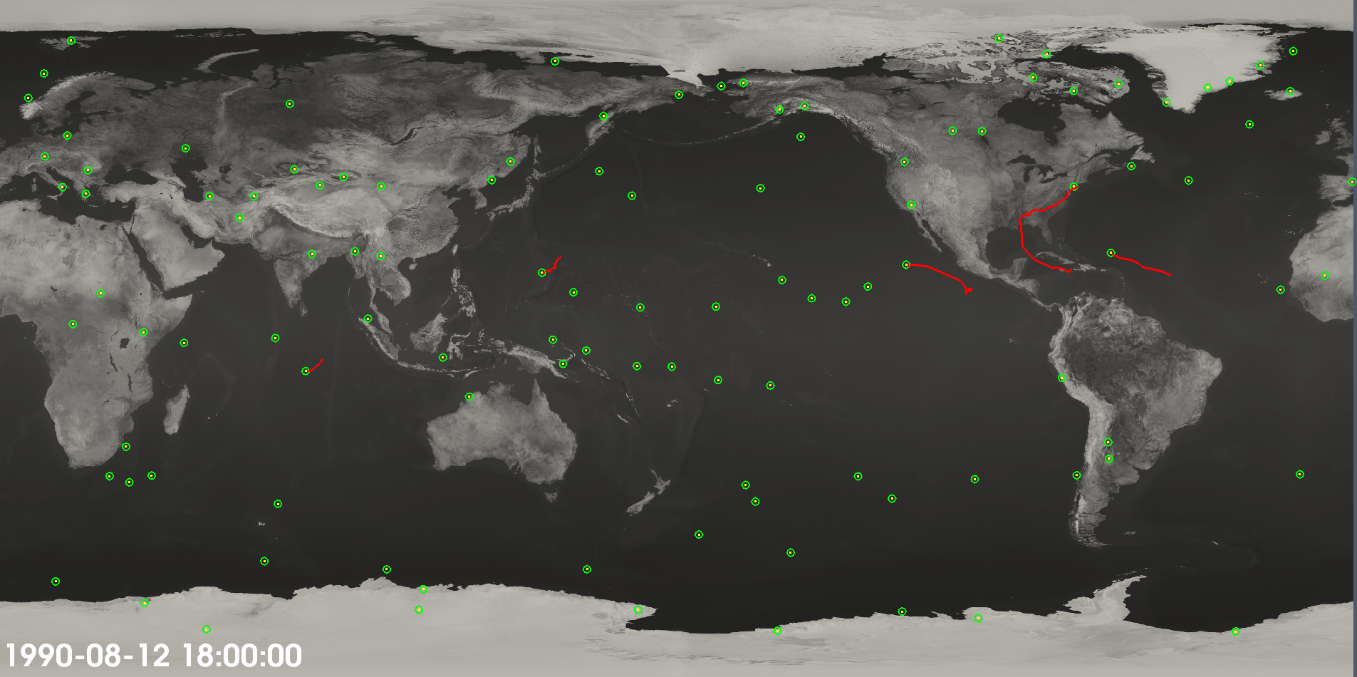
Fig. 2 Cyclone tracks plotted with 850 mb wind speed and integrated moisture.

Tropical Cyclone Detector¶

The cyclone detector is an MPI+threads parallel map-reduce based application that identifies tropical cyclone tracks in NetCDF-CF2 climate data. The application is comprised of a number of stages that are run in succession producing tables containing cyclone tracks. The tracks then can be visualized or further analyzed using the TECA TC statistics application, TECA’s Python bindings, or the TECA ParaView plugin.

Command Line Arguments¶

The most common command line options are:

--help

prints documentation for the most common options. MPI programs, such as teca_tc_detect aren’t allowed to run on the login noes at NERSC. For this reason to use textit{–help} you’ll need to obtain a compute node via textit{salloc} first.

–full_help: prints documentation for all options. See textit{–help} notes.
–input_regex: this is how you tell TECA what files are in the dataset. We use the grep style regex, which must be quoted with single ticks to protect it from the shell. Regex meta characters present in the file name must be escaped with a textbackslash. An example of an input regex which includes all .nc files is: ‘.*textbackslash.nc$’. If instead one wanted to grab only files from 2004-2005 then ‘.*textbackslash.200[45 .*textbackslash.nc$’ would do the trick. For the best performance, specify the smallest set of files needed to achieve the desired result. Each of the files will be opened in order to scan the time axis.
–start_date: an optional way to further specify the time range to process. The accepted format is a CF style human readable date spec such as YYYY-MM-DD hh:mm:ss. Because of the space in between day and hour spec quotes must be used. For example “2005-01-01 00:00:00”. Specifying a start date is optional, if none is given then all of the time steps in all of the files specified in the textit{–input_regex} are processed.
–end_date: see textit{–start_date}. this is has a similar purpose in restricting the range of time steps processed.
–candidate_file: a file name specifying where to write the storm candidates to. If not specified result will be written to candidates.bin in the current working directory. One sets the output format via the extension. Supported formats include csv, xlsx, and bin.
–track_file: a file name specifying where to write the detected storm tracks. If not specified the tracks are written to a file named tracks.bin in the current working directory. See textit{–candidate_file} for information about the supported formats.

Example¶

Once on Edison load the TECA module

module load teca

note that there are multiple versions installed, just use the latest and greatest as they become available.

Processing an entire dataset is straight forward once you know how many cores you want to run on. You will launch teca_tc_detect, the tropical cyclone application, from a SLURM batch script. A batch script is provided below.

TECA can process any size dataset on any number of compute cores. However, the fastest results are attained when there is 1 time step per core. In order to set this up one must determine how many time steps there are and write the SLURM batch script accordingly. The teca_metadata_probe command line application can be used for this purpose. When executed with the same textit{–input_regex} and optionally the textit{–start_date} and or textit{–end_date} options that will be used in the cyclone detection run it will print out the information needed to configure a 1 to 1 (time steps to cores) run. The metadata probe is a serial application and can be run on the login nodes.

teca_metadata_probe --input_regex '.*\.199[0-9].*\.nc$'

# A total of 29200 steps available in 3650 files. Using the noleap calendar.
# Times are specified in units of days since 1979-01-01 00:00:00. The available
# times range from 1990-1-1 3:0:0 (4015.12) to 2000-1-1 0:0:0 (7665).

With the number of time steps in hand one can set up the SLURM batch script for the run. The following batch script, named textit{1990s.sh}, processes the entire decade of the 1990’s. The teca_metadata_probe was used to determine that there are 29200 time steps. The srun command is used to launch the cyclone detector on 29200 cores.

#!/bin/bash -l

#SBATCH -p regular
#SBATCH -N 1217
#SBATCH -t 00:30:00

data_dir=/scratch2/scratchdirs/prabhat/TCHero/data
files_regex=cam5_1_amip_run2'\.cam2\.h2\.199[0-9].*.nc$'

srun -n 29200 teca_tc_detect                    \
    --input_regex ${data_dir}/${files_regex}    \
    --candidate_file candidates_1990s.bin       \
    --track_file tracks_1990s.bin

Finally, the batch script must be submitted to the batch system requesting the appropriate number of nodes. In this case the command is:

sbatch ./1990s.sh

For the $frac{1}{4}$ degree resolution dataset when processing latitudes between -90 to 90 the detector runs in approx 15 min. Detector run time could be reduced by subsetting in latitude (see textit{–lowest_lat}, textit{–highest_lat} options). Note that as the number of files in the dataset increases the metadata phase takes more time. You can use teca_metadata_probe to get a sense of how much more and extend the run time accordingly.

Tropical Cyclone Trajectories¶

Analyses produced by the stats stage¶

Table 1 Stats output 1¶
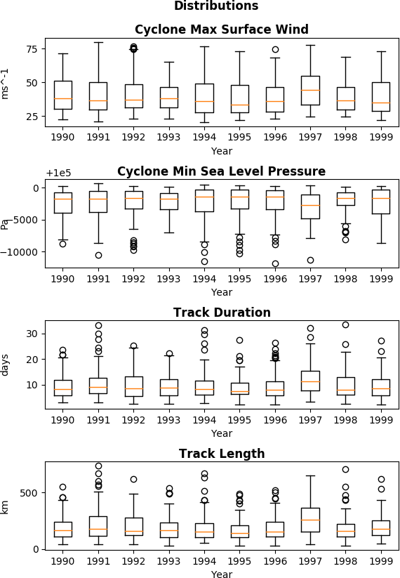
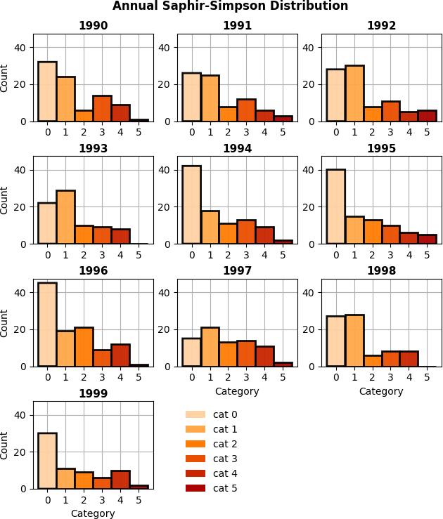
Fig. 3 Parameter Dist.	Fig. 4 Categorical Dist.
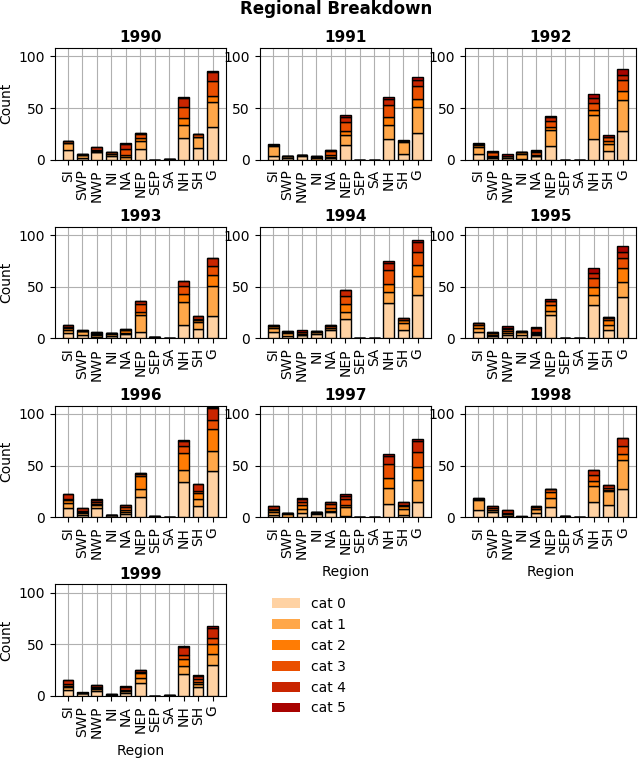
Fig. 5 Monthly Breakdown	Fig. 6 Regional Breakdown
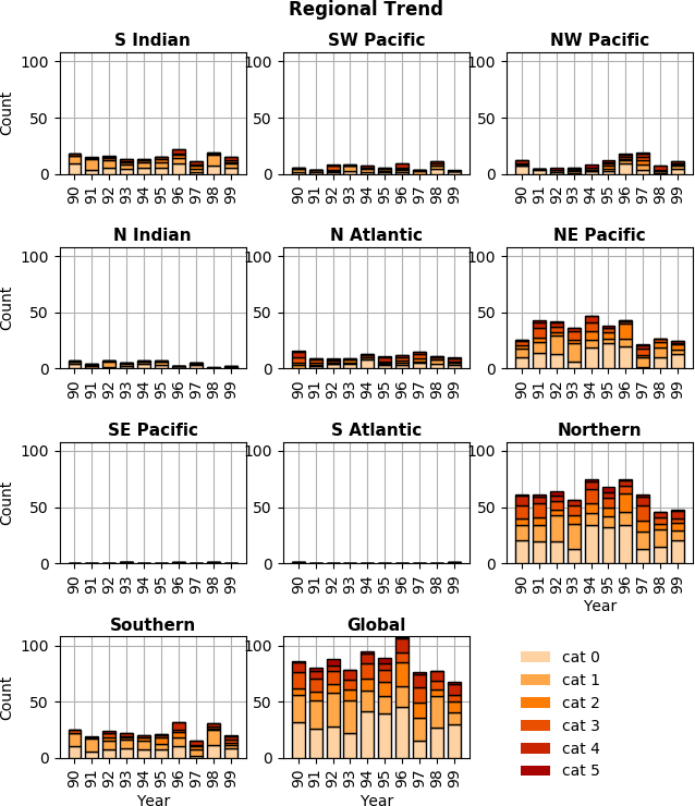
Fig. 7 Regional trend.

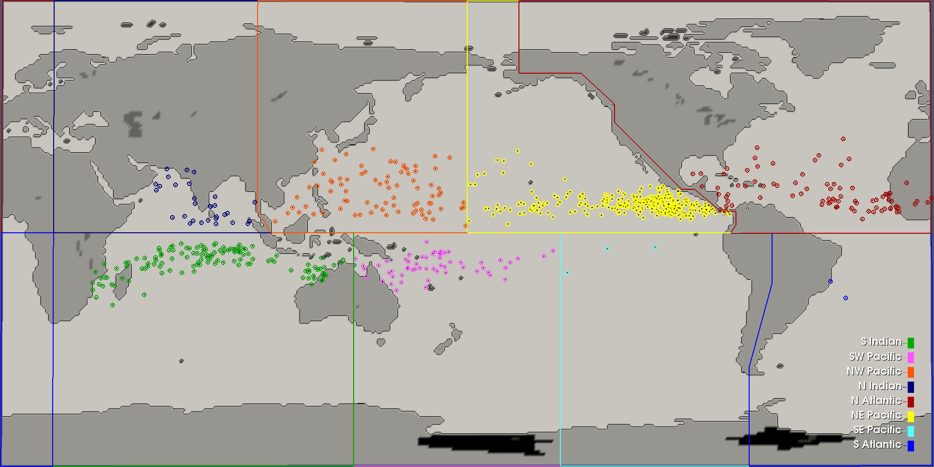
Fig. 8 Basin Definitions and Cyclogenesis Plot

The trajectory stage runs after the map-reduce candidate detection stage and generates cyclone storm tracks. The TC detector described above invokes the trajectory stage automatically, however it can also be run independently on the candidate stage output. The trajectory stage can be run from the login nodes.

Command Line Arguments¶

The most commonly used command line arguments to the trajectory stage are:

--help

prints documentation for the most common options.

–full_help: prints documentation for all options. See textit{–help} notes.
–candidate_file: a file name specifying where to read the storm candidates from.
–track_file: a file name specifying where to write the detected storm tracks. If not specified the tracks are written to a file named tracks.bin in the current working directory. One sets the output format via the extension. Supported formats include csv, xlsx, and bin.

Example¶

An example of running the trajectory stage is:

teca_tc_trajectory \
    --candidate_file candidates_1990s.bin       \
    --track_file tracks_1990s.bin

the file textit{tracks_1990s.bin} will contain the list of storm tracks.

TC Wind Radii¶

The wind radii application can be used to compute wind radii from track data in parallel. For each point on each track a radial profile is computed over a number of angular intervals. The radial profiles are used to compute distance from the storm center to the first downward crossing of given wind speeds. The default wind speeds are the3 Saffir-Simpson transitions. Additionally distance to the peak wind speed and peak wind speed are recorded. A new table is produced containing the data. The TC trajectory scalars application, TC stats application and ParaView plugin can be used to further analyze the data.

Command Line Arguments¶

The most commonly used command liine arguments are:

–track_file: file path to read the cyclone from (tracks.bin)
–wind_files: regex matching simulation files containing wind fields ()
–track_file_out: file path to write cyclone tracks with size (tracks_size.bin)
–wind_u_var: name of variable with wind x-component (UBOT)
–wind_v_var: name of variable with wind y-component (VBOT)
–track_mask: expression to filter tracks by ()
–n_theta: number of points in the wind profile in the theta direction (32)
–n_r: number cells in the wind profile in radial direction (32)
–profile_type: radial wind profile type. max or avg (avg)
–search_radius: size of search window in deg lat (6)

see –help and –full_help for more information.

Example¶

The following examples shows computation of wind radii for a decades worth of tracks using 128 cores on NERSC Cori.

module load teca
sbatch wind_radii_1990s.sh

where the contents of textit{wind_radii_1990s.sh} are as follows

#!/bin/bash -l
#SBATCH -p debug
#SBATCH -N 4
#SBATCH -t 00:30:00
#SBATCH -C haswell

data_dir=/global/cscratch1/sd/mwehner/cylones_ensemble/cam5_1_amip_run2/ncfiles
files_regex=${data_dir}/cam5_1_amip_run2'\.cam2\.h2\.199[0-9].*\.nc$'
track_file=tracks_1990s_3hr_mdd_4800.bin
track_file_out=wind_radii_1990s_3hr_mdd_4800_co.bin

srun -n 4 --ntasks-per-node=1 \
    teca_tc_wind_radii --n_threads 32 --first_track 0 \
    --last_track -1 --wind_files ${files_regex} --track_file ${track_file} \
    --track_file_out ${track_file_out}

Tropical Cyclone Statistics¶

The statistics stage can be used to compute a variety of statistics on detected cyclones. It generates a number of plots and tables and it can be ran on the login nodes. The most common options are the input file and output prefix.

Command Line Arguments¶

The command line arguments to the stats stage are:

tracks_file: A required positional argument pointing to the file containing TC storm tracks.
output_prefix: Required positional argument declaring the prefix that is prepended to all output files.

`--help`	prints documentation for the command line options.
`-d, --dpi`	Sets the resolution of the output images.
`-i, --interactive`
	Causes the figures to open immediately in a pop-up window.

-a, –ind_axes: Normalize y axes in the subplots allowing for easier inter-plot comparison.

Analysis¶

The following analysis are performed by the stats stage:

Classification Table: Produces a table containing cyclogenisis information, Saphir-Simpson category, and the min/max of a number of detection parameters.
Categorical Distribution: Produces a histogram containing counts of each class of storm on the Saphir-Simpson scale. See figure Fig. 4.
Categorical Monthly Breakdown: Produces histogram for each year that shows the breakdown by month and Saphir-Simpson category. See figure Fig. 5.
Categorical Regional Breakdown: Produces a histogram for each year that shows breakdown by region and Saphir-Simpson category. See figure Fig. 6.
Categorical Regional Trend: Produces a histogram for each geographic region that shows trend of storm count and Saphir-Simpson category over time. See figure Fig. 7
Parameter Distributions: Produces box and whisker plots for each year for a number of detector parameters. See figure Fig. 3.

Example¶

An example of running the stats stage is:

teca_tc_stats tracks_1990s.bin stats/stats_1990s

TC Trajectory Scalars¶

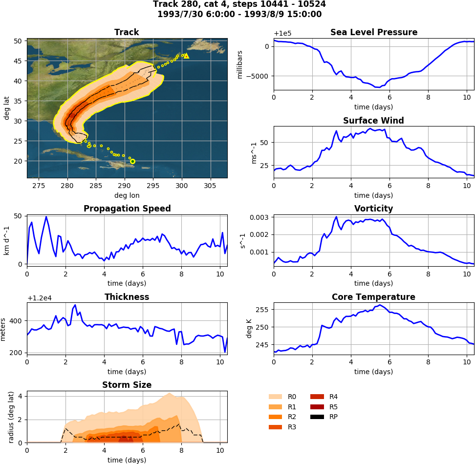
_images/track_scalars_1990s_3hr_mdd_4800_000280.png

Fig. 9 The trajectory scalars application plots cyclone properties over time.

The trajectory scalars application can be used to plot detection parameters for each storm in time. The application can be run in parallel.

Command Line Arguments¶

tracks_file: A required positional argument pointing to the file containing TC storm tracks.
output_prefix: A required positional argument declaring the prefix that is prepended to all output files.

`-h, --help`	prints documentation for the command line options.
`-d, --dpi`	Sets the resolution of the output images.
`-i, --interactive`
	Causes the figures to open immediately in a pop-up window.

–first_track: Id of the first track to process
–last_track: Id of the last track to process

--texture

An image containing a map of the Earth to plot the tracks on.

Example¶

mpiexec -np 10 ./bin/teca_tc_trajectory_scalars   \
    --texture ../../TECA_data/earthmap4k.png      \
    tracks_1990s_3hr_mdd_4800.bin                 \
    traj_scalars_1990s_3hr_mdd_4800

TC Wind Radii Stats¶

The wind radii stats application can be used to generate summary statistics describing the wind radii distributions.

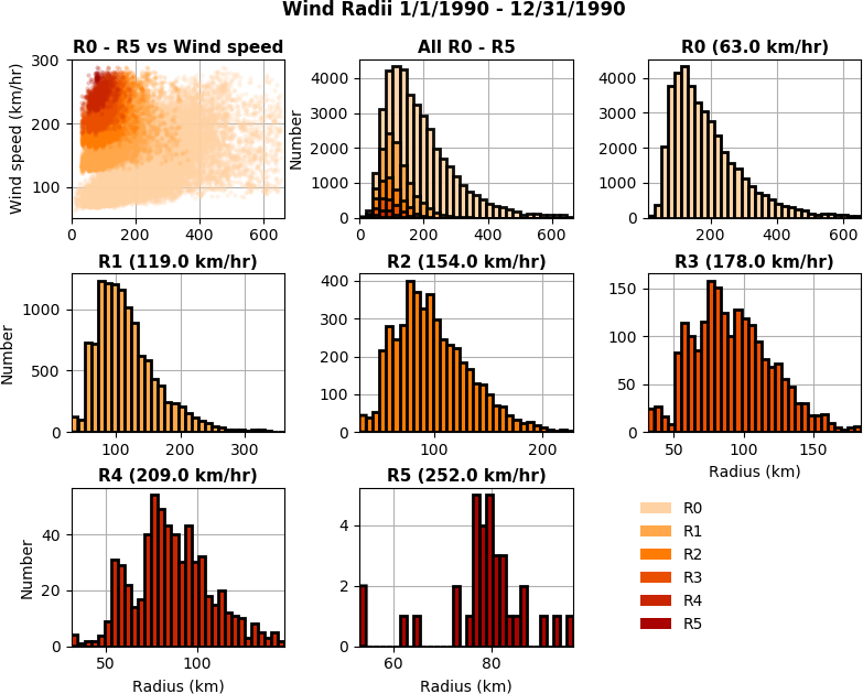
Fig. 10 The wind radii stats application plots distribution of wind radii.

Command Line Arguments¶

tracks_file: A required positional argument pointing to the file containing TC storm tracks.
output_prefix: Required positional argument declaring the prefix that is prepended to all output files.

`--help`	prints documentation for the command line options.
`-d, --dpi`	Sets the resolution of the output images.
`-i, --interactive`
	Causes the figures to open immediately in a pop-up window.

–wind_column: Name of the column to load instantaneous max wind speeds from.

Example¶

teca_tc_wind_radii_stats \
    wind_radii_1990s_3hr_mdd_4800_ed.bin wind_radii_stats_ed/

Event Filter¶

The event filter application lets one remove rows from an input table that do not fall within specified geographic and/or temporal bounds. This gives one the capability to zoom into a specific storm, time period, or geographic region for detailed analysis.

Command Line Arguments¶

in_file: A required positional argument pointing to the input file.
out_file: A required positional argument pointing where the output should be written.

-h, --help

prints documentation for the command line options.

–time_column: name of column containing time axis
–start_time: filter out events occurring before this time
–end_time: filter out events occurring after this time
–step_column: name of column containing time steps
–step_interval: filter out time steps modulo this interval
–x_coordinate_column: name of column containing event x coordinates
–y_coordinate_column: name of column containing event y coordinates
–region_x_coords: x coordinates defining region to filter
–region_y_coords: y coordinates defining region to filter
–region_sizes: sizes of each of the regions

Example¶

teca_event_filter --start_time=1750 --end_time=1850                       \
    --region_x_coords 260 320 320 260 --region_y_coords 10 10 50 50       \
    --region_sizes 4 --x_coordinate_column lon --y_coordinate_column lat  \
    candidates_1990s_3hr.bin filtered.bin