Python

TECA includes a diverse collection of I/O and analysis algorithms specific to climate science and extreme event detection. It’s pipeline design allows these component algorithms to be quickly coupled together to construct complex data processing and analysis pipelines with minimal effort. TECA is written primarily in C++ in order to deliver the highest possible performance and scalability. However, for non-computer scientists c+11 development can be intimidating, error prone, and time consuming. TECA’s Python bindings offer a more approachable path for custom application and algorithm development.

Python can be viewed as glue for connecting optimized C++ components. Using Python as glue gives one all of the convenience and flexibility of Python scripting with all of the performance of the native C++ code. TECA also includes a path for fully Python based algorithm development where the programmer provides Python callables that implement the desired analysis. In this scenario the use of technologies such as NumPy provide reasonable performance while allowing the programmer to focus on the algorithm itself rather than the technical details of C++ development.

Pipeline Components:

All of TECA’s pipeline stages are derived from the same base class. This makes them interchangeable and easy to use. However, when designing new pipelines and for understanding TECA’s parallel execution strategies it is useful to think about different types of pipeline stages.

Reader : A stage that presents data stored externally to the system, typically on disk, to the system and is capable of streaming subsets of the available data in parallel to the system on demand. The reader typically defines the control keys needed for parallel load balancing. Execution engines make use of these keys to parallelize execution automatically across MPI ranks, threads, and GPUs distributed on a HPC system. One of the primary jobs of the reader is efficiently creating a metadata view of what’s available without reading it all in. This is done so that runtime specified conditions unique to individual pipelines or datasets can be used to subset the data minimizing the amount of data pulled from storage. For example when detecting an AR, some detectors only need IVT, it would be wasteful to read other variables for that calculation. Each stage in the pipeline gets to specify the data it needs, the reader will provide only that data.

Writer : A stage that stores the data processed by the system to external storage media, typically disks. One of the primary jobs of the writer is to examine the available data and the set of files. Due to TECA’s parallel execution capabilities writers can be quite complex as they need to collectively route the large amounts of data streaming through the system on many nodes and threads to user defined file layouts such as daily, monthly, or yearly. For this reason writers often become execution engines driving capable of load balancing across MPI ranks, threads, and GPUs.

Processor : A stage that computes and makes a new quantity available to down stream stages. This is the most simple and most common stage type and includes operations such as computing norms, gradients, Laplacian, vorticity, connected component labeling, and so on. Processor stages should be designed to do compute a single quantity or do a single operation, do no I/O, and avoid communication. The first makes it easier to re-use common code, the latter two mean that I/O and parallelization do not interfere with parallelization, which is typically handled by execution engines connected down stream. When developing a new processor stage, focus on computing the new quantity on a single piece of data. The metadata view of the data can be used to determine specifics such as spatial or temporal coordinates if needed. Typically one need not think at all about parallelization. If one writes their processor to operate on a single piece of data, it can be parallelized automatically.

Transform : A stage that transforms the spatial or temporal coordinate system of the dataset. These stages must manipulate the view of the data that’s presented to the downstream and mediate requests for data in the new coordinate system to the original. These stages can sometimes become execution engines in that they may need to take control of the pipeline execution to fetch the needed data. One such example is the teca_temporal_reduction which transforms the time axis via a reduction operator, such as an average, over a run time specified interval such as monthly.

Execution Engine : A stage that is capable of examining the view of available data, partitioning work amongst the available compute nodes, MPI ranks, threads and GPUs, and then driving the pipeline in parallel. Execution engines make use of requests to which the upstream responds when driving the pipeline. In this way each time the pipeline runs it may process a different piece of the available data. Many of TECA’s execution engines are derived from the teca_threaded_algorithm, a stage that parallelizes over MPI, threads, and GPUs. The teca_threaded_algorithm uses a pool of threads to run the upstream pipeline once each for a set of run time defined requests. When developing a new execution engine derived from the teca_threaded_algorithm the primary task is providing this set of requests and processing the resulting data. Typically the downstream pipeline is single threaded to avoid a combinatorial explosion of threads that would ensue if multiple threaded algorithms were used in the same pipeline.

Reduction Engine : A specialized execution engine that takes N inputs and applies a reduction operation to produce a single output. The reduction engine typically makes us of threads, via the teca_trheaded_algrotihm, to drive the upstream pipeline in parallel when producing the N inputs. In that case the N inputs can arrive in a number and order to to the non-deterministic nature of threading. When the teca_threaded_algorithm’s streaming feature is enabled, a reduction may specify the minimum number of inputs it can process by setting the stream size property. The inputs are processed in chunks equal to the stream size. Streaming overlaps the reduction with the calculation of the N inputs and reduces memory use compared to processing all N inputs simultaneously. The teca_index_reduce is a base class containing all of the logic for parallelizing and streaming execution over a set of requests. One implements an override top generate a set of requests and an override to perform the reduction of 2 inputs to produce a single output. The teca_index_reduce is the easiest way to implement new reductions. A second example is the teca_temporal_reduction. This stage transforms the time axis from one interval to another via a reduction operator.

The list of above types is an arbitrary way of thinking about the system that is often useful for new users wishing to stitch together custom pipelines and develop new pipeline stages. However, keep in mind that in the case of more complex operations the lines between the above types become blurred. User’s must take care when multiple execution/reduction engines are connected in the same pipeline. Typically only one of the engines may use threading.

Parallel Execution

TECA pipelines are designed for parallel execution on multi-node high performance computing systems and will automatcially parallelize work across nodes, MPI ranks, threads and GPUs.

Index set : Data is presented to the system as a set of indices. Using an idex set to represent the data makes it possible to parallelize across diverse input data types using the same execution engines. For instance the index set may represent the time steps of a climate simulation, or spatial tiles of a single time step, or a collection of events such as cyclone or AR detections.

The pipeline runs once for each index to be processed. During pipeline execution, an execution engine or executive generates a light weight request that specifies the index to be processed as well as any other subsetting information such as a list of necessary variables, or spatial bounds. An upstream stage, typically the reader, responds to this request providing the requested data. Subsequent stages process the data as needed.

Executive : There are two pathways to parallel execution in TECA: execution engines and executives. Executives implement a simple form of parallelism and provide a means for runtime execution control such as runtime defined spatial, temporal, and data subsetting. Executives are presented with a view of the available data, and a combination of runtime settings, from which they create requests for each piece of data to be processed. The teca_index_executive parallelizes requests across MPI ranks.

Execution Engines : Execution engines are pipeline stages that manipulate pipeline requests to take control of pipeline execution. Execution engines implement threading and parallelize work across MPI ranks, threads, and GPUs.

Job size : When running TECA in parallel one must choose the number of MPI ranks to use. TECA is capable of running any job on any number of MPI ranks. However, when fewer MPI ranks are used than there are available work, i.e. indices in the index set, some or all MPI ranks will process multiple indices sequentially. The total run time of the job will be the largest number of indices processed by all ranks times the time it takes to process a single index. When the number of MPI ranks does not divide the number of indices evenly some MPI ranks will be idle in the last pass over the data. Likewise, when there are more MPI ranks than there are available work (indices in the index set) some MPI ranks will have no work. For these reasons it is advisable to size MPI jobs such that each MPI rank has the same number of indices to process, and to estimate the total runtime when MPI ranks have more than one to process to ensure that the job is given sufficient runtime.

Climate Data Specific Execution Patterns

A number of execution patterns have been implemented that enable data to be processed in parallel.

Index Parallelism : This is the most generic and flexible mode where indices in the index set are mapped onto MPI ranks, threads, and GPUs. The indices may be time steps of the simulation, the individual steps of a cyclone track, or something else. There are no restrictions on what the indices represent. This parallel mode is available in the teca_threaded_algorithm, teca_cf_writer, teca_temporal_reduction, teca_index_reduce, teca_table_reduce and teca_index_executive.

Temporal Parallelism : In this case the indices are the time steps of the input dataset. All of the data associated with a single time step is processed in a single pipeline execution. This parallel mode is available in the same classes listed under index parallelism.

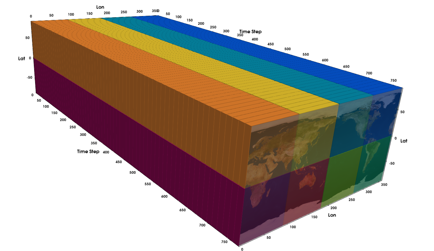
Fig. 15 With spatial parallelism work is mapped to hardware over a number of spatio-temporal domains such that each MPI rank is responsible for a unique set of spatial regions across all time steps. In this example there are 8 spatial partitions, 8 MPI ranks, and 768 time steps partitioned into blocks of 12 timesteps.

Spatial Parallelism : This case is specific to spatio-temporal data on Cartesian meshes. the input domain is partitioned in to a runtime specified number of spatial and temporal partitions. The partitions are then assigned cyclically to MPI ranks such that each MPI rank is responsible for a given spatial subset over all times. The temporal domain may be partitioned into either a run time specified number of partitions or partitions of a given size. The amount of parallelism attainable in this mode is limited by the number of spatial partitions, the time domain partitions are processed sequentially.

When the number of spatial partitions is equal to the number of MPI ranks, the MPI ranks will process the same temporal partition per pipeline execution. When the number of temporal partitions is set to one the entire time history of a given spatial region is processed at together. See figure Fig. 15 for an example.

This mode is available in the teca_spatial_executive and the teca_cf_writer.

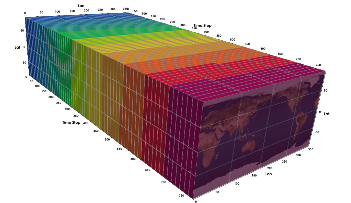
Fig. 16 With space-time parallelism work is mapped to hardware over a number of spatio-temporal domains. When there is only a single spatial partition this mode is equivalent to

Sace-Time Parallelsm : This case is specific to spatio-temporal data on Cartesian meshes. the input domain is partitioned in to a runtime specified number of spatial and temporal partitions. The partitions are then assigned to MPI ranks in contiguous blocks such that each MPI rank processes approximately the same number of partitions. The temporal domain may be partitioned into either a run time specified number of partitions or into partitions of a given size. The parallelism attainable in this mode of execution is limited by the product of the number of spatial and temporal partitions.

When there is a single spatial partition and the size of the temporal partitions is one, execution is equivalent to temporal parallelization. See figure Fig. 16 for an example.

This mode is available in the teca_space_time_executive and the teca_cf_writer.

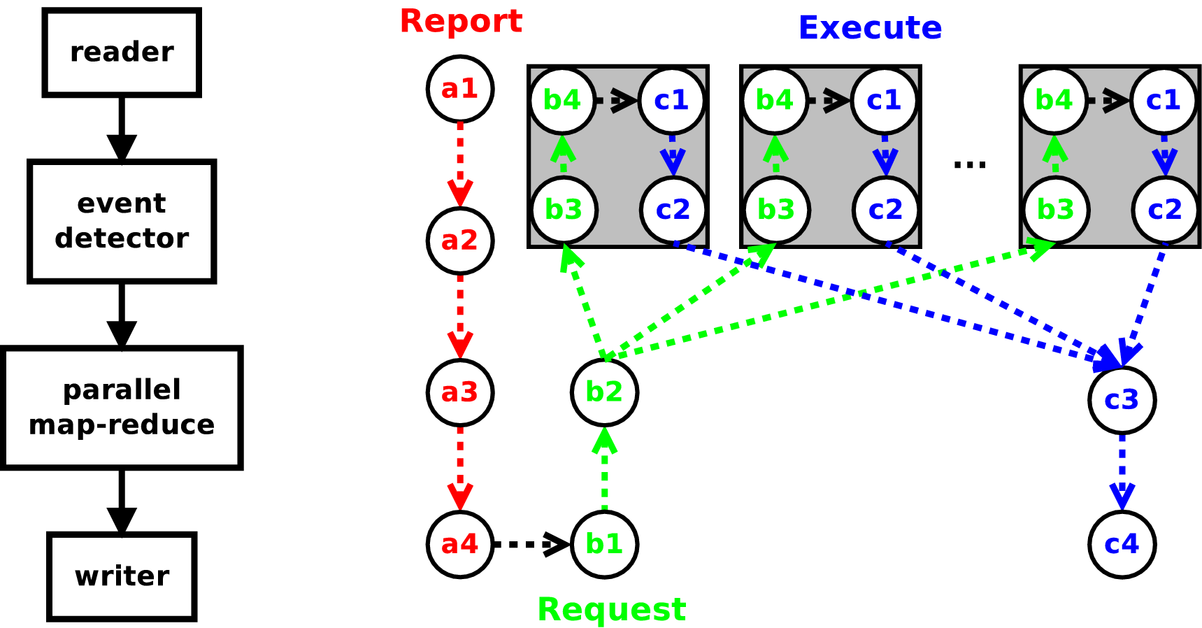
Fig. 17 execution path through a simple 4 stage pipeline on any given process in an MPI parallel run. Time progresses from a1 to c4 through the three execution phases report (a), request (b), and execute (c). The sequence of thread parallel execution is shown inside gray boxes, each path represents the processing of a single request.

Pipeline Construction, Configuration and Execution

Building pipelines in TECA is as simple as creating and connecting TECA algorithms together in the desired order. Data will flow and be processed sequentially from the top of the pipeline to the bottom, and in parallel where parallel algorithms are used. All algorithms are created by their static New() method. The connections between algorithms are made by calling one algorithm’s set_input_connection() method with the return of another algorithm’s get_output_port() method. Arbitrarily branchy pipelines are supported. The only limitation on pipeline complexity is that cycles are not allowed. Each algorithm represents a stage in the pipeline and has a set of properties that configure its run time behavior. Properties are accessed by set_<prop name>() and get_<prop name>() methods. Once a pipeline is created and configured it can be run by calling update() on its last algorithm.

Listing 1 Command line application written in Python. The application constructs, configures, and executes a 4 stage pipeline that computes basic descriptive statistics over the entire lat-lon mesh for a set of variables passed on the command line. The statistic computations have been written in Python, and are shown in listing Listing 2. When run in parallel, the map-reduce pattern is applied over the time steps in the input dataset. A graphical representation of the pipeline is shown in figure Fig. 17

from mpi4py import *
from teca import *
import sys
from stats_callbacks import descriptive_stats

if len(sys.argv) < 7:
    sys.stderr.write('global_stats.py [dataset regex] ' \
        '[out file name] [first step] [last step] [n threads]' \
        '[array 1] .. [ array n]\n')
    sys.exit(-1)

data_regex = sys.argv[1]
out_file = sys.argv[2]
first_step = int(sys.argv[3])
last_step = int(sys.argv[4])
n_threads = int(sys.argv[5])
var_names = sys.argv[6:]

if MPI.COMM_WORLD.Get_rank() == 0:
    sys.stderr.write('Testing on %d MPI processes\n'%(MPI.COMM_WORLD.Get_size()))

cfr = teca_cf_reader.New()
cfr.set_files_regex(data_regex)

alg = descriptive_stats.New()
alg.set_input_connection(cfr.get_output_port())
alg.set_variable_names(var_names)

mr = teca_table_reduce.New()
mr.set_input_connection(alg.get_output_port())
mr.set_thread_pool_size(n_threads)
mr.set_start_index(first_step)
mr.set_end_index(last_step)

tw = teca_table_writer.New()
tw.set_input_connection(mr.get_output_port())
tw.set_file_name(out_file)

tw.update()

For example, listing Listing 1 shows a command line application written in Python. The application computes a set of descriptive statistics over a list of arrays for each time step in the dataset. The results at each time step are stored in a row of a table. teca_table_reduce is a map-reduce implementation that processes time steps in parallel and reduces the tables produced at each time step into a single result. One use potential use of this code would be to compute a time series of average global temperature. The application loads modules and initializes MPI (lines 1-4), parses the command line options (lines 6-17), constructs and configures the pipeline (lines 22-37), and finally executes the pipeline (line 39). The pipeline constructed is shown in figure Fig. 17 next to a time line of the pipeline’s parallel execution on an arbitrary MPI process.

Algorithm Development

While TECA is is written in C++, it can be extended at run time using Python. However, before we explain how this is done one must know a little about the three phases of execution and what is expected to happen during each.

The heart of TECA’s pipeline implementation is the teca_algorithm. This is an abstract class that contains all of the control and execution logic. All pipelines in TECA are built by connecting concrete implementations of teca_algorithm together to form execution networks. TECA’s pipeline model is based on a report-request scheme that minimizes I/O and computation. The role of reports are to make known to down stream consumers what data is available. Requests then are used to pull only the data that is needed through the pipeline. Requests enable subsetting and streaming of data and can be acted upon in parallel and are used as keys in the pipeline’s internal cache. The pipeline has 3 phases of execution, report phase, the request phase, and finally the execute phase.

Report Phase : The report phase kicks off a pipeline’s execution and is initiated when the user calls update() or update_metadata() on a teca_algorithm. In the report phase, starting at the top of the pipeline working sequentially down, each algorithm examines the incoming report and generates outgoing report about what it will produce. Implementing the report phase can be as simple as adding an array name to the list of arrays or as complex as building metadata describing a dataset on disk. The report phase should always be light and fast. In cases where it is not, cache the report for re-use. Where metadata generation would create a scalability issue, for instance parsing data on disk, the report should be generated on rank 0 and broadcast to the other ranks.

Request Phase : The request phase begins when report the report phase reaches the bottom of the pipeline. In the request phase, starting at the bottom of the pipeline working sequentially up, each algorithm examines the incoming request, and the report of what’s available on its inputs, and from this information generates a request for the data it will need during its execution phase. Implementing the request phase can be as simple as adding a list of arrays required to compute a derived quantity or as complex as requesting data from multiple time steps for a temporal computation. The returned requests are propagated up after mapping them round robin onto the algorithm’s inputs. Thus, it’s possible to request data from each of the algorithm’s inputs and to make multiple requests per execution. Note that when a threaded algorithm is in the pipeline, requests are dispatched by the thread pool and request phase code must be thread safe.

Execute Phase : The execute phase begins when requests reach the top of the pipeline. In the execute phase, starting at the top of the pipeline and working sequentially down, each algorithm handles the incoming request, typically by taking some action or generating data. The datasets passed into the execute phase should never be modified. When a threaded algorithm is in the pipeline, execute code must be thread safe.

In the TECA pipeline the report and request execution phases handle communication in between various stages of the pipeline. The medium for these exchanges of information is the teca_metadata object, an associative containers mapping strings(keys) to arrays(values). For the stages of a pipeline to communicate all that is required is that they agree on a key naming convention. This is both the strength and weakness of this approach. On the one hand, it’s trivial to extend by adding keys and arbitrarily complex information may be exchanged. On the other hand, key naming conventions can’t be easily enforced leaving it up to developers to ensure that algorithms play nicely together. In practice the majority of the metadata conventions are defined by the reader. All algorithms sitting down stream must be aware of and adopt the reader’s metadata convention. For most use cases the reader will be TECA’s NetCDF CF 2.0 reader, teca_cf_reader. The convention adopted by the CF reader are documented in its header file and in section ref{sec:cf_reader}.

In C++ and Python polymorphism is used to provide customized behavior for each of the three pipeline phases. In Python we use the teca_python_algorithm, an adapter class that connects the user provided overrides such that they are called at the appropriate times during each phase of pipeline execution. Hence writing a TECA algorithm purely in Python amounts to providing three appropriate overrides.

Listing 2 Overrides implementing the calculation of descriptive statistics over a set of variables laid out on a Cartesian lat-lon mesh. The request override requests the variables, the execute override makes the computations and constructs a table to store them in.

from mpi4py import MPI
from teca import *
import numpy as np
import sys

class descriptive_stats(teca_python_algorithm):

    def __init__(self):
        self.rank = MPI.COMM_WORLD.Get_rank()
        self.var_names = []

    def set_variable_names(self, vn):
        self.var_names = vn

    def request(self, port, md_in, req_in):
        sys.stderr.write('descriptive_stats::request MPI %d\n'%(self.rank))
        req = teca_metadata(req_in)
        req['arrays'] = self.var_names
        return [req]

    def execute(self, port, data_in, req):
        sys.stderr.write('descriptive_stats::execute MPI %d\n'%(self.rank))

        mesh = as_teca_cartesian_mesh(data_in[0])

        table = teca_table.New()
        table.declare_columns(['step','time'], ['ul','d'])
        table << mesh.get_time_step() << mesh.get_time()

        for var_name in self.var_names:

            table.declare_columns(['min '+var_name, 'avg '+var_name, \
                'max '+var_name, 'std '+var_name, 'low_q '+var_name, \
                'med '+var_name, 'up_q '+var_name], ['d']*7)

            var = mesh.get_point_arrays().get(var_name).as_array()

            table << np.min(var) << np.average(var) \
                << np.max(var) << np.std(var) \
                << np.percentile(var, [25.,50.,75.])

        return table

Python Algorithm Template

To extend TECA using Python one derives from teca_python_algorithm. A template follows:

class YOUR_CLASS_NAME(teca_python_algorithm):

    # YOUR INITIALIZATION CODE

    # YOUR PROPERTY SETTING CODE

    def report(self, o_port, reports_in):
        # YOUR CODE REPORTING NEW DATA PRODUCED IN
        # EXECUTE.

    def request(self, o_port, reports_in, request_in):
        # YOUR CODE REQUESTING SPECIFIC DATA NEEDED
        # IN EXECUTE

    def execute(self, o_port, data_in, request_in):
        # YOUR CODE DO A CALCULATION, TRANSFORM DATA,
        # OR MAKING A SIDE AFFECT

One overrides one por more of the three methods: report, request, and execute. In addition one can add initialization and properties that control run time behavior. For instance a writer may use a file_name property to specify the locatgion on disk to put the data. Typically this would be accessed via a set_file_name method. The overrides are described in more detail below.

The Report Override

The report override will report the universe of what the algorithm could produce.

def report(self, o_port, reports_in) -> report_out

o_port

integer. the output port number to report for. can be ignored for single output algorithms.

reports_in

teca_metadata list. reports describing available data from the next upstream algorithm, one per input connection.

report_out

teca_metadata. the report describing what you could potentially produce given the data described by reports_in.

Report stage should be fast and light. Typically the incoming report is passed through with metadata describing new data that could be produced appended as needed. This allows upstream data producers to advertise their capabilities.

The Request Override

The request override generates an up stream request requesting the minimum amount of data actually needed to fulfill the incoming request.

def request(self, o_port, reports_in, request_in) -> requests_out

o_port

integer. the output port number to report for. can be ignored for single output algorithms.

reports_in

teca_metadata list. reports describing available data from the next upstream algorithm, one per input connection.

request_in

teca_metadata. the request being made of you.

report_out

teca_metadata list. requests describing data that you need to fulfill the request made of you.

Typically the incoming request is passed through appending the necessary metadata as needed. This allows down stream data consumers to request data that is produced upstream.

The Execute Override

The execute override is where the computations or I/O necessary to produce the requested data are handled.

def execute(self, o_port, data_in, request_in) -> data_out

o_port

integer. the output port number to report for. can be ignored for single output algorithms.

data_in

teca_dataset list. a dataset for each request you made in the request override in the same order.

request_in

teca_metadata. the request being made of you.

data_out

teca_dataset. the dataset containing the requested data or the result of the requested action, if any.

A simple strategy for generating derived quantities having the same data layout, for example on a Cartesian mesh or in a table, is to pass the incoming data through appending the new arrays. This allows down stream data consumers to receive data that is produced upstream. Because TECA caches data it is important that incoming data is not modified, this convention enables shallow copy of large data which saves memory.

Lines 25-27 of listing Listing 1 illustrate the use of teca_python_algorithm. In this example a class derived from teca_python_algorithm computes descriptive statistics over a set of variables laid out on a Cartesian lat-lon mesh. The derived class, descriptive_stats, is in a separate file, stats_overrides.py (listing Listing 2) imported on line 4.

Listing Listing 2 shows the class derived from teca_python_algorithm that is used in listing Listing 1. The class implements request and execute overrides. Note, that we did not need to provide a report override as the default implementation, which passes the report through was all that was needed. Our request override (lines 15-21 of listing Listing 2) simply adds the list of variables we need into the incoming request which it then forwards up stream. The execute override (lines 23-45) gets the input dataset (line 27), creates the output table adding columns and values of time and time step (lines 29-31), then for each variable we add columns to the table for each computation (line 35), get the array from the input dataset (line 39), compute statistics and add them to the table (lines 41-43), and returns the table containing the results (line 45). This data can then be processed by the next stage in the pipeline.

Working with TECA’s Data Structures

Arrays

TODO: illustrate use of teca_variant_array, and role numpy plays

Metadata

TOOD: illustrate use of teca_metadata

The Python API for teca_metadata models the standard Python dictionary. Metadata objects are one of the few cases in TECA where stack based allocation and deep copying are always used.

md = teca_metadata()
md['name'] = 'Land Mask'
md['bounds'] = [-90, 90, 0, 360]

md2 = teca_metadata(md)
md2['bounds'] =  [-20, 20, 0, 360]

Array Collections

TODO: illustrate teca_array_collection, tabular and mesh based datasets are implemented in terms of collections of arrays

Tables

TODO: illustrate use of teca_table

Cartesian Meshes

TODO: illustrate use of teca_cartesian_mesh

NetCDF CF Reader Metadata

TODO: document metadata conventions employed by the reader